10 Jul 2026
 Planet Python
Mike Driscoll: An Intro to Spiel – Creating Presentations in Your Terminal with Python
Have you ever wanted to create a presentation in your computer's terminal? While this is an uncommon need, a clever open source developer has provided a solution to this problem! The project is called Spiel, and while it is currently archived, the idea is pretty cool. Spiel uses the Rich package to create the slides for your presentation. Note: while the GitHub page doesn't explain why the project is archived, it appears to use a very old version of Textual which cannot be upgraded.
Let's spend a little time learning how this all works.
Installing Spiel
According to the Spiel GitHub page, you can try Spiel without even installing it if you have docker installed. Here's how to try Spiel:
$ docker run -it --rm ghcr.io/joshkarpel/spiel
However, for the purposes of this tutorial, you really should install Spiel. To do that, you will be using pip. Open up your terminal and run the following:
pip install spiel
Feel free to create a Python virtual environment first if you don't want to install Spiel into your global Python packages.
Once you have Spiel installed, you can check that it is working by running the Spiel demo, like this:
spiel demo present
If that works, you are good to go!
Creating Your Presentation
The documentation gives a good example of how to create a one-slide presentation. Here's their example:
from rich.console import RenderableType

from spiel import Deck, present

deck = Deck(name="Your Deck Name")


@deck.slide(title="Slide 1 Title")
def slide_1() -> RenderableType:
    return "Your content here!"


if __name__ == "__main__":
    present(__file__)
According to the documentation, there are two ways to add slides:
- Use the decorator like in the example above
- Use `deck.add_slides()` and pass in one or more Slide objects
Here is a more complete example that creates a couple of custom slides:
from rich.align import Align
from rich.console import RenderableType
from rich.style import Style
from rich.text import Text
from spiel import Deck, Slide, present


def make_slide(
    title_prefix: str,
    text: Text,
) -> Slide:
    def content() -> RenderableType:
        return Align(text, align="center", vertical="middle")
    return Slide(title=f"{title_prefix} Slide", content=content)

deck = Deck("Test Deck")

title_slide = make_slide(title_prefix="First", text=Text("Python 101 - All About Lists",
                                             style=Style(color="blue")))

intro_slide = make_slide(title_prefix="Second",
                    text=Text("A Python list is",
                              style=Style(color="red"))
                    )

deck.add_slides(title_slide, intro_slide)

if __name__ == "__main__":
    present(__file__)
When you run this code in your terminal, you will see something like this:
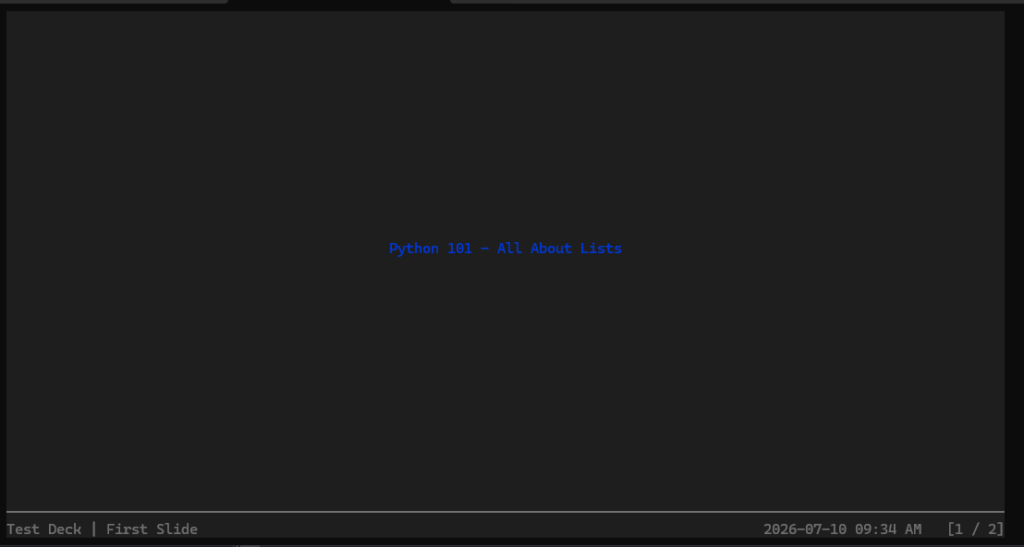
You can move to the next or previous slide using the arrow keys on your keyboard. If you want to exit, press CTRL+C.
Wrapping Up
Spiel seems like a neat package. It's a shame that it is currently archived. Hopefully, the author will reopen it at some point, or someone else will pick up the torch. In the meantime, you can easily use it in a Python virtual environment and give it a try.
The post An Intro to Spiel - Creating Presentations in Your Terminal with Python appeared first on Mouse Vs Python.
10 Jul 2026 3:13pm GMT
Talk Python to Me: #554: Trustworthy AI in Healthcare and Longevity
You ask an AI a question and it answers with total confidence. Most of the time, a confidently wrong answer is just an annoyance. But what if the question is medical, and there's a real patient on the other end? In that world, a hallucination isn't a bug, it's a patient-safety event. Sumit Gundawar is a London-based software engineer who builds the clinical platform for a UK longevity and aesthetic-medicine clinic, and his whole argument is that in high-stakes AI, the model is the easy part. Earning trust is the real engineering. We dig into grounding, refusal logic, human-in-the-loop design, and the messy frontier of longevity and biohacking, plus a live demo of an assistant that refuses to answer when it can't back up the claim. Let's get into it.<br/> <br/> <strong>Episode sponsors</strong><br/> <br/> <a href='https://talkpython.fm/sixfeetup'>Six Feet Up</a><br> <a href='https://talkpython.fm/training'>Talk Python Courses</a><br/> <br/> <h2 class="links-heading mb-4">Links from the show</h2> <div><strong>Guest</strong><br/> <strong>Sumit Gundawar</strong>: <a href="https://www.linkedin.com/in/sumit-gundawar-759470129/?featured_on=talkpython" target="_blank" >linkedin.com</a><br/> <br/> <strong>Course transcripts announcement</strong>: <a href="https://talkpython.fm/blog/posts/announcing-german-subtitles-on-courses/" target="_blank" >talkpython.fm/blog</a><br/> <br/> <strong>Sumit Gundawar - JAX London Speaker</strong>: <a href="https://jaxlondon.com/speaker/sumit-gundawar/?featured_on=talkpython" target="_blank" >jaxlondon.com</a><br/> <strong>Anthropic</strong>: <a href="https://anthropic.com/?featured_on=talkpython" target="_blank" >anthropic.com</a><br/> <strong>OpenAI Platform</strong>: <a href="https://platform.openai.com/?featured_on=talkpython" target="_blank" >platform.openai.com</a><br/> <strong>Anthropic</strong>: <a href="https://anthropic.com/?featured_on=talkpython" target="_blank" >anthropic.com</a><br/> <strong>LangChain</strong>: <a href="https://langchain.com/?featured_on=talkpython" target="_blank" >langchain.com</a><br/> <strong>OWASP</strong>: <a href="https://owasp.org/?featured_on=talkpython" target="_blank" >owasp.org</a><br/> <strong>Pydantic</strong>: <a href="https://pydantic.dev/?featured_on=talkpython" target="_blank" >pydantic.dev</a><br/> <strong>EU AI Act - Regulatory Framework</strong>: <a href="https://digital-strategy.ec.europa.eu/en/policies/regulatory-framework-ai?featured_on=talkpython" target="_blank" >digital-strategy.ec.europa.eu</a><br/> <strong>HIPAA - HHS</strong>: <a href="https://www.hhs.gov/hipaa?featured_on=talkpython" target="_blank" >www.hhs.gov</a><br/> <strong>NHS</strong>: <a href="https://www.nhs.uk/?featured_on=talkpython" target="_blank" >www.nhs.uk</a><br/> <strong>Llama</strong>: <a href="https://llama.com/?featured_on=talkpython" target="_blank" >llama.com</a><br/> <strong>Qwen - QwenLM on GitHub</strong>: <a href="https://github.com/QwenLM?featured_on=talkpython" target="_blank" >github.com</a><br/> <strong>OpenAI Platform</strong>: <a href="https://platform.openai.com/?featured_on=talkpython" target="_blank" >platform.openai.com</a><br/> <strong>Hugging Face</strong>: <a href="https://huggingface.co/?featured_on=talkpython" target="_blank" >huggingface.co</a><br/> <strong>Llama</strong>: <a href="https://llama.com/?featured_on=talkpython" target="_blank" >llama.com</a><br/> <strong>Granola</strong>: <a href="https://www.granola.ai/?featured_on=talkpython" target="_blank" >www.granola.ai</a><br/> <strong>HIPAA - HHS</strong>: <a href="https://www.hhs.gov/hipaa?featured_on=talkpython" target="_blank" >www.hhs.gov</a><br/> <strong>CodeRabbit</strong>: <a href="https://www.coderabbit.ai/?featured_on=talkpython" target="_blank" >www.coderabbit.ai</a><br/> <strong>Cursor Origin</strong>: <a href="https://cursor.com/origin?featured_on=talkpython" target="_blank" >cursor.com</a><br/> <strong>GitHub Status</strong>: <a href="https://www.githubstatus.com/?featured_on=talkpython" target="_blank" >www.githubstatus.com</a><br/> <strong>Midjourney Medical</strong>: <a href="https://www.midjourney.com/medical?featured_on=talkpython" target="_blank" >www.midjourney.com</a><br/> <strong>Neko Health</strong>: <a href="https://www.nekohealth.com/?featured_on=talkpython" target="_blank" >www.nekohealth.com</a><br/> <strong>CERN</strong>: <a href="https://home.cern/?featured_on=talkpython" target="_blank" >home.cern</a><br/> <strong>ATLAS Experiment</strong>: <a href="https://atlas.cern/?featured_on=talkpython" target="_blank" >atlas.cern</a><br/> <br/> <strong>Watch this episode on YouTube</strong>: <a href="https://www.youtube.com/watch?v=pp2v9paEoq4" target="_blank" >youtube.com</a><br/> <strong>Episode #554 deep-dive</strong>: <a href="https://talkpython.fm/episodes/show/554/trustworthy-ai-in-healthcare-and-longevity#takeaways-anchor" target="_blank" >talkpython.fm/554</a><br/> <strong>Episode transcripts</strong>: <a href="https://talkpython.fm/episodes/transcript/554/trustworthy-ai-in-healthcare-and-longevity" target="_blank" >talkpython.fm</a><br/> <br/> <strong>Theme Song: Developer Rap</strong><br/> <strong>🥁 Served in a Flask 🎸</strong>: <a href="https://talkpython.fm/flasksong" target="_blank" >talkpython.fm/flasksong</a><br/> <br/> <strong>---== Don't be a stranger ==---</strong><br/> <strong>YouTube</strong>: <a href="https://talkpython.fm/youtube" target="_blank" ><i class="fa-brands fa-youtube"></i> youtube.com/@talkpython</a><br/> <br/> <strong>Bluesky</strong>: <a href="https://bsky.app/profile/talkpython.fm" target="_blank" >@talkpython.fm</a><br/> <strong>Mastodon</strong>: <a href="https://fosstodon.org/web/@talkpython" target="_blank" ><i class="fa-brands fa-mastodon"></i> @talkpython@fosstodon.org</a><br/> <strong>X.com</strong>: <a href="https://x.com/talkpython" target="_blank" ><i class="fa-brands fa-twitter"></i> @talkpython</a><br/> <br/> <strong>Michael on Bluesky</strong>: <a href="https://bsky.app/profile/mkennedy.codes?featured_on=talkpython" target="_blank" >@mkennedy.codes</a><br/> <strong>Michael on Mastodon</strong>: <a href="https://fosstodon.org/web/@mkennedy" target="_blank" ><i class="fa-brands fa-mastodon"></i> @mkennedy@fosstodon.org</a><br/> <strong>Michael on X.com</strong>: <a href="https://x.com/mkennedy?featured_on=talkpython" target="_blank" ><i class="fa-brands fa-twitter"></i> @mkennedy</a><br/></div>
10 Jul 2026 5:10am GMT
09 Jul 2026
Planet Python
EuroPython: Humans of EuroPython: Daria Linhart Grudzień
EuroPython wouldn&apost exist without the wonderful volunteers who pour countless hours into organising it. From contracting the venue to selecting and confirming talks and workshops, hundreds of hours of loving work go into making each edition the best one yet.
Join us in celebrating one of the humans behind the keyboard. Today, we&aposre delighted to share an interview with Daria Linhart Grudzień, our Communications Lead.
Thank you for being the voice of the EuroPython community, Daria!

EP: What first inspired you to volunteer for EuroPython? And which edition of the conference was it?
I got pulled into the team in 2025, tempted with a chance to work with a friend on organising an event for juniors in tech in Czechia, which became the Beginners Day Unconference. I appreciated that a major European conference offered a program for the local community.
EP: Did you make any lasting friendships or professional connections through volunteering?
Lots! The EuroPython team is full of kind and fun people who like to do interesting things in their free time. Being a member of the core organising team gave me a chance to get to know a lot of folks. For the first time I feel like I'm going to the conference to meet up with friends.
EP: What was your primary role as a volunteer, and what did a typical day of contributing look like for you?
After doing the Humans of EuroPython interviews during the winter, I got invited to lead the Communications Team for the 2026 edition. My days include a variety of tasks,which I love. From building a productive team, working on finding media partners, occasional web development, co-ordinating with other teams, building documentation for the next edition, to making sure folks in the team enjoy contributing - I do what's needed to make sure EuroPython speaks to our community with a friendly, slightly quirky, but always inclusive voice.
EP: Was there a moment when you felt your contribution really made a difference?
There were a few. Some of the core Python developers reached out to me personally saying that the Communications Team is doing a great job. Seeing our social media posts engage and resonate with the community is another reminder that our work is making an impact.
EP: Would you volunteer again, and why?
Absolutely. Contributing to EuroPython, I feel empowered to bring ideas, experiment, and work on impactful initiatives which benefit the community. I've been able to take on roles and projects which allowed me to learn, get out of my comfort zone, and grow. I hope to do more of that in the future, and this is a fantastic group of people to do this with.
EP: If you could describe the volunteer experience in three words, what would they be?
Ownership. Impact. Collaboration.
EP: Did you have any unexpected or funny experiences at EuroPython?
I got invited to talk about the conference on the Real Python Podcast. This wasn't on my bingo card for this year 🙂
09 Jul 2026 5:05pm GMT
Python Software Foundation: The PSF D&I Workgroup Are Starting Office Hours in July!

Starting Tuesday 28 July, 2026, the PSF Diversity & Inclusion (D&I) Workgroup is opening its virtual doors once a month on Discord. Come chat with workgroup members from all over the world!
Doing diversity and inclusion work in tech can feel isolating sometimes. You might be organizing a meetup, writing a code of conduct, trying to get funding for your community, or helping people feel welcome, often in your spare time, and wondering if anyone else is wrestling with the same things.
They are. We are! And we would love to get all of us in the same room.
This July, the PSF D&I Workgroup will be hosting monthly office hours within Discord. These will be open, text-based conversations where we encourage you to ask questions, sha
re what you are working on, and connect with other people who care about making the Python community more welcoming.
The details
The PSF D&I Office Hours will be on the last Tuesday of every month. Because our community is spread across the globe, we will alternate between two times so we can cover as many time zones as possible:
-
1 PM UTC / 9 AM US Eastern
-
9 PM UTC / 5 PM US Eastern
Our first session will be on Tuesday, 28 July 2026 at 1 PM UTC. Here is roughly what that looks like around the world:
|
Region |
Local time on 28 July |
|
US Pacific, Los Angeles - (UTC-7h) |
6:00 AM |
|
US Eastern, New York - (UTC-4h) |
9:00 AM |
|
Brazil, São Paulo - (UTC-3h) |
10:00 AM |
|
UTC |
1:00 PM |
|
West Africa, Lagos - (UTC+1h) |
2:00 PM |
|
Central Europe, Amsterdam / Berlin / Madrid - (UTC+2h) |
3:00 PM |
|
East Africa, Nairobi - (UTC+3h) |
4:00 PM |
|
Iran, Tehran - (UTC+3:30h) |
4:30 PM |
|
India, New Delhi - (UTC+5:30h) |
6:30 PM |
|
China, Beijing - (UTC+8h) |
9:00 PM |
|
Japan, Tokyo - (UTC+9h) |
10:00 PM |
|
Australia, Sydney - (UTC+10h) |
11:00 PM |
If 6 AM in Los Angeles or 11 PM in Sydney made you wince, do not worry. The August session will be at 9 PM UTC, and we will keep alternating from there.
You will find us in the #psf-diversity channel on the PSF Discord. If you're new to Discord, check out some Discord Basics to help you get started.
What will we talk about
Honestly? Whatever is on your mind related to Python, your communities, and D&I.
Since our workgroup exists to advise the PSF on diversity and inclusion, some conversations we are especially hoping to have include:
-
Ideas for policies, initiatives, and grant proposals to diversify the PSF missions. Feedback from the community about these topics will help the PSF D&I Workgroup provide recommendations to the PSF Board of Directors.
-
Your feedback, plain and simple. We want to understand how the PSF can better serve and grow a diverse membership, and we cannot do that without hearing from the community itself.
-
How things are actually going. Part of our job is measuring and sharing the PSF's progress on its diversity initiatives, and we would rather do that in conversation with you than in a report nobody reads. We also want to understand and learn about the current state of Python communities around the world.
No camera, no mic, no pressure
Office hours are text chat only.
Show up in your pajamas, join from the bus, lurk quietly for the first twenty minutes. It is all fine.
And if you cannot make it at all, the conversation stays in the channel, so you can catch up later when it suits you. If something in the chat sparks a thought you would like to share with us directly, you are always welcome to email the workgroup at diversity-inclusion-wg@python.org.
Bring your own language
Because we are the D&I Workgroup, our members come from around the world! Alongside the main conversation, we will open threads in other languages where possible. Depending on the presence of our members, we would be happy to chat in Spanish, Portuguese, Chinese, Hindi, French or even Persian! Let us know during the office hour if you have a specific language you hope to converse in, or jump in with whichever language thread feels like home.
See you on the 28th!
The first office hour session is on Tuesday, 28 July 2026 at 1 PM UTC, in #psf-diversity on Discord.
Come say hi, even if it is just to tell us what you are working on with Python. We are really looking forward to meeting you!
09 Jul 2026 2:11pm GMT
08 Jul 2026
Planet Python
Django Weblog: Last Call 2026 Django Developer Survey
Time is running out. This is the last call for the 2026 Django Developers Survey, which the Django Software Foundation is running in partnership with JetBrains.
The survey closes on July 13, 2026. It is one of the best measures we have of how Django is used, and it helps guide future technical and community decisions.
So far, over 3,100 people have responded, and we would love to push that number past 4,000. Every response helps us better understand the Django community.
This year's survey was shaped by the Django Steering Council, the Django Fellows, the Django Software Foundation Board of Directors, and several community members. Your feedback helps us understand your needs, see how you use Django, and plan for future development and community needs.
How you can help
Once you've done the survey, take a moment to re-share on socials and with your communities. The more diverse the answers, the better the results for all of us. We appreciate everybody helping to get the word out.
Please use the following links:
-
Bluesky
https://surveys.jetbrains.com/s3/bs-django-developers-survey-2026 -
Django Forum
https://surveys.jetbrains.com/s3/df-django-developers-survey-2026 -
LinkedIn
https://surveys.jetbrains.com/s3/li-django-developers-survey-2026 -
Mastodon
https://surveys.jetbrains.com/s3/md-django-developers-survey-2026 -
Reddit
https://surveys.jetbrains.com/s3/r-django-developers-survey-2026 -
X / Twitter
https://surveys.jetbrains.com/s3/x-django-developers-survey-2026
For more details, read the original announcement on the Django blog.
08 Jul 2026 7:31pm GMT
Mike Driscoll: New Book Release: Python Typing
I am happy to announce that my latest book, Python Typing, is now available on all platforms. You can get your copy on Gumroad or Leanpub or Amazon
Python has had type hinting support since Python 3.5, over TEN years ago! However, Python's type annotations have changed repeatedly over the years. In Python Typing: Type Checking for Python Programmers, you will learn all you need to know to add type hints to your Python applications effectively.
You will also learn how to use Python type checkers, configure them, and set them up in pre-commit or GitHub Actions. This knowledge will give you the power to check your code and your team's code automatically before merging, hopefully catching defects before they make it into your products.
What You'll Learn
You will learn all about Python's support for type hinting (annotations). Specifically, you will learn about the following topics:
- Variable annotations
- Function annotations
- Type aliases
- New types
- Generics
- Hinting callables
- Annotating TypedDict
- Annotating Decorators and Generators
- Using Mypy for type checking
- Mypy configuration
- Using ty for type checking
- ty configuration
- and more!
Where to Purchase
The post New Book Release: Python Typing appeared first on Mouse Vs Python.
08 Jul 2026 6:46pm GMT
Hugo van Kemenade: Fixing the dictionary with Python 3.14
Yes, but not the dict kind of dictionary.
When working on CPython, we often find obscure bugs elsewhere, in compilers, operating systems and elsewhere:
Since Python 3.8, the release notes have a section called "And now for something completely different". These have included Monty Python sketches, astrophysics facts and poetry.
For Python 3.14, I'm doing all things π, pie and [mag]pie (more here). As part of the research for this important task, I looked up pi in the Oxford English Dictionary.
As we all recall from the Python 3.14.0b1 release notes, William Jones was the first person to use the π symbol to denote the circle's circumference to its diameter in his Synopsis Palmariorum Matheseos (1706):

However, the OED's first citation had a markup bug:
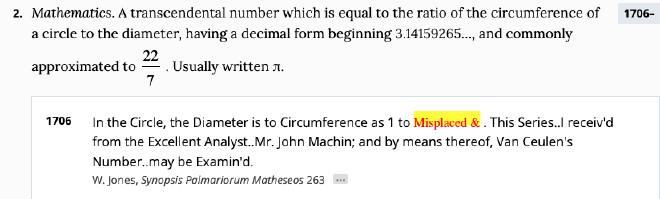
I duly reported this to the OED in July 2024; and by the next time I looked it up, in June 2025, it was fixed!
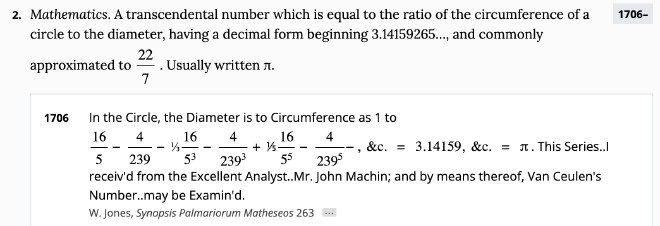
Hooray!
Header photo: Part of the definition for "get" in the OED's 1901 forerunner, A New English Dictionary on Historical Principles (CC BY-NC-SA 2.0 Hugo van Kemenade).
08 Jul 2026 4:40pm GMT
Marc-André Lemburg: My 25th EuroPython - in a row😊

Next weekend, I&aposll be heading to Kraków, Poland, for my 25th EuroPython conference.
It&aposs been a long ride since the first EuroPython conference in Charleroi, Belgium, but one I wouldn&apost have wanted to miss.
This year, I&aposll be giving a talk about DuckLake, an extension to DuckDB, one of the most exciting new database systems in the last few years.
Come join in.
Cheers,
Marc-André
08 Jul 2026 3:48pm GMT
Python GUIs: Why Widgets Appear as Separate Windows — Understanding widget parenting in Qt and how to fix widgets that float outside your main window
Sometimes when I dynamically add widgets to tabs in my PyQt6 application, they pop out as windows instead. What's going on?
If you're dynamically adding widgets to your PyQt6 application and finding that they pop out as separate floating windows instead of appearing neatly inside your application, you're running into one of Qt's gotchas: widget parenting.
This problem usually shows up when widgets are added from a callback, event listener or signal handler. But there are a million different ways to screw this up. Let's look at why this happens and how to fix it.
How Qt decides what's a window
In Qt, every widget can optionally have a parent widget. The parent determines where a widget lives visually - a widget with a parent is drawn inside that parent. A widget without a parent becomes a top-level window, floating independently on your desktop.
This is the root cause of widgets appearing outside your main window. When you create a widget and it doesn't have a parent - either because you didn't set one, or because the parent was lost somehow - Qt treats it as a standalone window.
Three ways to Get a Parent-less Widget
Here are the most common reasons widgets end up floating:
Creating widgets without a parent
# This widget has no parent - it will be a floating window
tabs = QTabWidget()

# This widget has a parent - it will appear inside parent_widget
tabs = QTabWidget(parent_widget)
When you add a widget to a layout, the layout assigns the parent automatically. But if something goes wrong between creation and layout insertion (like an exception, or the widget being shown prematurely), the widget stays parentless.
The safest approach is to pass a parent when creating widgets:
def create_new_tab(self):
    wdg = QWidget()
    layout = QGridLayout(wdg)

    tabs = QTabWidget(wdg)  # Explicitly set parent
    tab1 = QWidget(tabs)     # Explicitly set parent
    tab2 = QWidget(tabs)     # Explicitly set parent
    tabs.addTab(tab1, "Start")
    tabs.addTab(tab2, "Profile")
    layout.addWidget(tabs)

    return wdg
...although, honestly, I don't usually bother. If I know I'll be adding a widget to a layout immediately, I'll omit the parent assignment.
In an window __init__ the safety question is less relevant because, if there is an unhandled exception that blocks the adding your sub-widget to a layout, it will also block the creation of the parent window.
Accidentally recreating a widget
If you have a tab widget stored as self.w and somewhere in your code you do:
self.w = QTabWidget()
...the original tab widget is replaced. If the old widget gets garbage collected, all the tabs that had it as their parent suddenly become orphans - parentless widgets that float as independent windows.
Be careful not to reassign widget attributes unintentionally, especially in callbacks that might run multiple times.
Losing the parent reference
If you explicitly set a widget's parent to None, it becomes a top-level window:
widget.setParent(None) # This widget is now a floating window
This sometimes happens indirectly. For example, removing a widget from a layout in certain ways can clear its parent.
A clean approach to dynamic tabs
Here's a complete, working example that dynamically adds tabs without any floating-window issues. It demonstrates the correct way to set up a QTabWidget with a "+" button that adds new tabs:
import sys
from PyQt6.QtWidgets import (
    QApplication, QMainWindow, QTabWidget,
    QWidget, QVBoxLayout, QLabel
)


class MainWindow(QMainWindow):
    def __init__(self):
        super().__init__()
        self.setWindowTitle("Dynamic Tabs")
        self.setFixedSize(600, 400)

        self.tabs = QTabWidget(self)
        self.tabs.currentChanged.connect(self.on_tab_changed)

        # Add an initial tab
        self.add_content_tab("Tab 1")

        # Add the "+" tab for creating new tabs
        self.tabs.addTab(QWidget(self.tabs), "+")

        self.setCentralWidget(self.tabs)

    def on_tab_changed(self, index):
        # Check if the "+" tab was clicked
        if self.tabs.tabText(index) == "+":
            self.add_new_tab()

    def add_new_tab(self):
        # Count existing content tabs (exclude the "+" tab)
        tab_count = self.tabs.count()  # includes "+"
        new_title = f"Tab {tab_count}"

        # Insert the new tab before the "+" tab
        new_tab = self.create_tab_content(new_title)
        insert_index = self.tabs.count() - 1
        self.tabs.insertTab(insert_index, new_tab, new_title)

        # Switch to the newly created tab (avoid retriggering)
        self.tabs.blockSignals(True)
        self.tabs.setCurrentIndex(insert_index)
        self.tabs.blockSignals(False)

    def add_content_tab(self, title):
        """Add a content tab before the + tab."""
        tab = self.create_tab_content(title)
        # Insert before the last tab if "+" exists, otherwise just add
        plus_index = None
        for i in range(self.tabs.count()):
            if self.tabs.tabText(i) == "+":
                plus_index = i
                break

        if plus_index is not None:
            self.tabs.insertTab(plus_index, tab, title)
        else:
            self.tabs.addTab(tab, title)

    def create_tab_content(self, title):
        """Create the widget content for a tab."""
        widget = QWidget(self.tabs)  # Parent is the tab widget
        layout = QVBoxLayout(widget)
        label = QLabel(f"Content for {title}", widget)
        layout.addWidget(label)
        return widget


app = QApplication(sys.argv)
window = MainWindow()
window.show()
sys.exit(app.exec())
A few things to notice in this example:
- The main window inherits from
QMainWindow, andQApplicationis created separately. - Every widget is created with an explicit parent:
QWidget(self.tabs),QLabel(text, widget), etc. blockSignals(True)is used when programmatically changing the current tab to prevent thecurrentChangedsignal from firing recursively.- New tabs are inserted before the "+" tab using
insertTab, so the "+" always stays at the end.
Summary
Widget parenting is one of those things in Qt that works invisibly when everything is correct - and causes confusing visual glitches the moment something is slightly off. The good news is that once you understand the pattern, the fix is almost always the same: make sure every widget has a parent.
If you're new to PyQt6, our guide to creating your first window covers the basics of setting up a QMainWindow, while the widgets tutorial walks through the most common widgets and how to use them correctly.
For an in-depth guide to building Python GUIs with PyQt6 see my book, Create GUI Applications with Python & Qt6.
08 Jul 2026 6:00am GMT
07 Jul 2026
Planet Python
Brett Cannon: How to publish to PyPI using GitHub Actions securely
There have been several security incidents lately that involved compromising GitHub Actions workflows. This has led some to say "GitHub Actions is the weakest link" in publishing and to GitHub publishing a GitHub Actions security roadmap update. But saying it&aposs an issue and acknowledging the fact is one thing, but you still need to do the mitigation work today so you are not going to be the next headline. So this post is going to outline 3 things to do so you can publish to PyPI securely when using GitHub Actions.
But before I go any farther, I want to make 2 things very clear. One is this post is in no way meant to shame anyone into using GitHub Actions. For instance, I have heard people trying to shame maintainers into using GitHub Actions to use Trusted Publishing, and I think that&aposs wrong. Now, if you choose to use a platform that supports Trusted Publishing, then you should definitely use it. But Trusted Publishing is not a reason to change your publishing workflow if the one you have is already secure. In other words, use whatever works best for you to publish securely to PyPI, and if that&aposs GitHub Actions then this blog post is for you.
Two, the title of this post explicitly says "publishing" and not "building and publishing". Doing builds securely is a separate concern that I am not covering. The one piece of advice I will give, though, is one the Python security developer in residence gave me: you should have building and publishing be separate workflows.
With that out of the way, here are 3 steps to securing GitHub Actions for publishing to PyPI that should be relatively painless.
Use zizmor
The zizmor tool examines your GitHub Actions workflows to find things that at dubious when it comes to security. They pretty much all stem from GitHub Actions having insecure defaults in the name of convenience. There are 2 parts to using zizmor:
- Make it happy
- Set it up in CI
You can do those two things in whatever order you want but you need to do both to make sure you fix any current issues you have and prevent any new issues from slipping in. Luckily both things are easy to do.
Make zizmor happy
To run zizmor you can do uvx zizmor --quiet --fix .github/ , pipx zizmor --quiet --fix .github/ , or however you choose to run it. That will run zizmor and fix anything that it can in a clean way. Chances are, though, there will be three things to fix by hand.
No permissions by default
By default, the token GitHub Actions gives to your workflow via GITHUB_TOKEN is way too broad, so zizmor flags it. Easiest way to fix this issue is to turn off all permissions at the global level for a workflow and then turn any permissions you need on at the job level. So put the following at the global level of your workflow file (I personally put it just before jobs:):
permissions: {}If you happen to need some specific permission, you can then specify it per-job so you scope it as tightly as possible. Or if you really need something for everything, you can still set it globally, but you at least you will be explicit about exactly what you want.
The reason you do this is you don&apost want some action to get a hold of your token that can do something as if you&aposre you and do something bad.
No persisted credentials after checkout
When you use the checkout action, GitHub Actions is running Git on your behalf, complete with credentials so the git checkout command works. The problem is those credentials persist passed the checkout action unless you specifically say to not keep them around. So add the following with: clause to your checkout action:
  with:
    persist-credentials: false
You do this so your credentials don&apost leak out to some action that will do something bad with them.
Pin your actions
When you specify an action to use in a workflow, you were probably told to use some Git tag like uses: actions/checkout@v7 which specifies using the v7 tag from the https://github.com/actions/checkout repo. The problem with that is if that action gets compromised, an attacker can just update that tag to point to malicious code and so now you&aposre compromised.
You work around this by pinning your actions to commit hashes. This might sound like a massive hassle, but there are tools that can pin all your actions for you.
- gha-update
zizmor --fix --gh-tokenwith a (permissionless) token- Pinact
Those go from simplest to fanciest, but they all get the job done. I personally use gha-update as it&aposs quick and updates my versions along the way. But if you want to keep your current versions as-is then zizmor will do it for you, but you need to give it a token to do the updates (the token is required to avoid being throttled by GitHub). The best thing to do is to use a permissionless token, but if you&aposre being lazy and trust zizmor (and any tool you might be using to run it, e.g. uvx), you can get a token from gh auth token (the following example is for the Fish shell; adjust the syntax for calling gh accordingly for your shell and how you prefer to call zizmor):
zizmor --quiet --fix --gh-token (gh auth token) .githubIf you need fancier than any of that, use Pinact.
You also want to require pinning not only for your workflows but any actions that use actions themselves so you&aposre pinned top to bottom. The easiest way to make that a requirement is to run the following command:
gh api "/repos/{owner}/{repo}/actions/permissions" --method PUT --field enabled=true --field sha_pinning_required=trueThere&aposs also a way to do it via the UI:
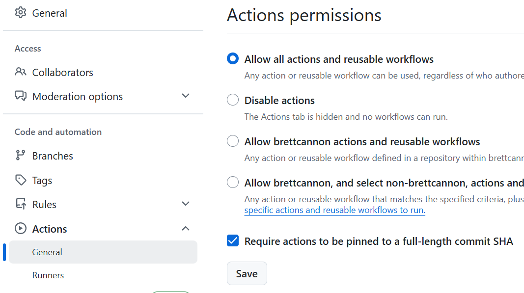 Screenshot of turning on required SHA pinning in a repo under Settings - Actions - General
Bonus: Dependabot to keep actions up-to-date
Dependabot will recognize your use of pins, so you can still use it to keep your actions up-to-date (if you so choose; it&aposs okay if you don&apost want to use Dependabot). The one thing I suggest is using a cooldown so you don&apost accidentally pick to a malicious update by adding a cooldown of a week to your dependabot.yml:
- package-ecosystem: github-actions
  directory: /
  schedule:
    interval: monthly
  cooldown:
    default-days: 7
Add zizmor to CI
Conveniently, zizmor has an action you can set up in your repo. Using it will cause any issues found to be reported as a code scanning result under the "Security and quality" tab (which can be turned off).
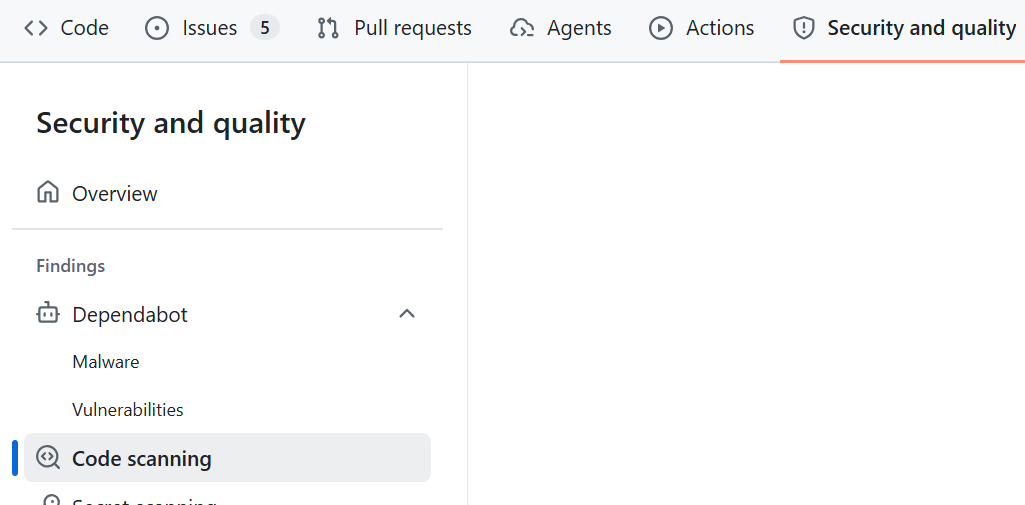 Screenshot showing the "Code scanning" view under the "Security and quality" tab on GitHub
This means the results are private and thus you don&apost have to worry about exposing anything publicly. You can also use the results as a TODO list if you would find that more motivating to have something to check off instead of getting everything working upfront. As well, if you want to do it gradually this will give you a checklist of things to fix.
You can also run zizmor manually if you want in CI, but I personally just use the zizmor action in a dedicated workflow since the zizmor docs provide such a workflow configuration.
Use Trusted Publishing
If you&aposre going to use GitHub Actions to publish to PyPI, I don&apost see any reason not to use Trusted Publishing. It means you don&apost have to manage any API tokens and you can get attestations. Basically it means you get to outsource your security concerns for how you communicate with PyPI for publishing to GitHub&aposs security team.
The one thing you should make sure to do when setting up Trusted Publishing is set up a GitHub environment. The Trusted Publishing docs strongly encourage it and so do I. You can even have the environment do nothing, but doing it now at least gives you an easy option to use it for something later. But I do suggest you use environments to ...
Require approval to publish
The one specific thing I suggest you do with your GitHub environment is require reviewers to run your publishing workflow. The required reviewer can be yourself! But the key point is to require someone to approve the workflow to run.
You might be wondering what&aposs the point if you trigger the release yourself? It&aposs to add a gate to protect against accidental running of your publishing workflow. The accident could be from you or it could be from a malicious actor who has managed to trigger the workflow. By requiring your approval, neither scenario can happen without you clicking that approval button while logged into your GitHub account. And that means someone would need to hack your GitHub account to work around it (and as mentioned above, that means you get to lean on the GitHub security team from preventing that from happening).
Out of everything I have listed, this is probably the most arduous as it&aposs a cost every time you want to do a release. But it&aposs one approval and you&aposre probably already going to be doing something to trigger the release, so you&aposre already online.
And that&aposs it! Those 3 steps get you a long way towards publishing securely from GitHub Actions to PyPI.
Acknowledgments
Thanks to Seth Larson for providing feedback on a draft of this post and giving advice on Mastodon when I posted about these steps. Thanks to William Woodruff for creating zizmor and also giving advice on Mastodon. And thanks to everyone who participated constructively in the discussion on Mastodon.
07 Jul 2026 8:44pm GMT
PyCoder’s Weekly: Issue #742: Wagtail as Admin, Random Values, Code Quality, and More (2026-07-07)
#742 - JULY 7, 2026
View in Browser »

Wagtail as Django Admin on Steroids
Wagtail can do pretty much everything the Django Admin can do, but includes a much more modern UI and more features. This article shows you how to use Wagtail as an Admin alternative.
TIM KAMANIN
Selecting Random Values in Python
Python's random module provides utilities for generating pseudorandom numbers. For cryptographically-secure randomness, use the secrets module instead.
TREY HUNNER
Let AI Agents Into Your B2B App. Securely.
More of your users are asking to connect AI agents to your product, and you want to say yes. PropelAuth lets you give each agent scoped, revocable access, so you stay in control of what it can do. Learn more →
PROPELAUTH sponsor
Managing and Measuring Python Code Quality
Master Python code quality tools like linters, formatters, type checkers, and profilers to measure, manage, and improve the code you write.
REAL PYTHON course
Discussions
Articles & Tutorials
Thinking About Running for the PSF Board? Let's Talk!
The Python Software Foundation Board has announced two office-hour sessions dedicated to giving information on running for the PSF Board. If you're thinking of running in the upcoming election, these sessions can help you understand the ins and outs.
PYTHON SOFTWARE FOUNDATION
Celery on AWS ECS: Complete Guide
Running Celery on AWS ECS without losing tasks and making sure that all the work is done is not as straightforward as it may seem. Learn how to configure Celery and structure your tasks for reliable processing.
JAN GIACOMELLI • Shared by Špela Giacomelli
Learn the Agentic Coding Workflow That Actually Works on Real Projects
65% of Python developers are stuck using AI for small tasks that fall apart on anything real. This 2-day live course (July 11-12 via Zoom) walks you through building a complete Python app with OpenAI's Codex, from an empty directory to a shipped project on GitHub. See the Full Curriculum →
REAL PYTHON sponsor
Free-Threaded Python: Past, Present, and Future
This post summarizes a talk by core developer Thomas Wouters at PyCon US 2026 on Free-threaded Python: the attempt to remove the GIL. It describes why it is being done and what future work looks like.
JAKE EDGE
In Search of a New Contribution Model
This opinion piece from Carlton Gibson, a core Django contributor, talks about the state of contributions to OSS, how AI has made them more complicated, and how some key things are still broken.
CARLTON GIBSON
How to Get TIFF MetaData With Python
The Pillow image library gives you lots of tools for dealing with images. This article teaches you how to extract metadata from TIFF files in a few lines of Python.
MIKE DRISCOLL
Profile First: A 10x Faster Django Test Suite
Bob's Django test suite took 30 seconds. cProfile showed 83% of it was one function: password hashing. Here's how he found the bottleneck and the five-line fix.
BOB BELDERBOS
Python 3.15 Preview: Upgraded JIT Compiler
Learn how the upgraded Python 3.15 JIT compiler speeds up your code with a new tracing frontend, register allocation, and in-place numeric operations.
REAL PYTHON
Store Extra Data for Objects in a WeakKeyDictionary
In several programs Adam has wanted to solve the problem of associating extra data with an object. This article outlines his latest approach.
ADAM JOHNSON
How to Get Started With the GitHub Copilot CLI
Learn how to install, authenticate, and use the GitHub Copilot CLI to plan, write, and review Python code from your terminal with AI agents.
REAL PYTHON
Projects & Code
pytest-tia: Run Only the Tests Your Git Diff Actually Affects
GITHUB.COM/BREADMSA • Shared by BreadWasEaten
purejq: A Pure-Python Implementation of jq
GITHUB.COM/ADAM2GO • Shared by adam2go
Events
Python Atlanta
July 9 to July 10, 2026
MEETUP.COM
PyDelhi User Group Meetup
July 11, 2026
MEETUP.COM
DFW Pythoneers 2nd Saturday Teaching Meeting
July 11, 2026
MEETUP.COM
EuroPython 2026
July 13 to July 20, 2026
EUROPYTHON.EU
SciPy 2026
July 13 to July 20, 2026
SCIPY.ORG
EuroSciPy 2026
July 18 to July 24, 2026
EUROSCIPY.ORG
Happy Pythoning!
This was PyCoder's Weekly Issue #742.
View in Browser »
[ Subscribe to 🐍 PyCoder's Weekly 💌 - Get the best Python news, articles, and tutorials delivered to your inbox once a week >> Click here to learn more ]
07 Jul 2026 7:30pm GMT
PyCharm: Best Object Detection Models for Machine Learning in 2026
Object detection powers transformative applications, from autonomous vehicles navigating city streets and security systems identifying threats in real time to retail analytics tracking inventory and medical imaging detecting tumors. But choosing the right model for your computer vision project can be challenging, especially with dozens of architectures claiming superiority across different metrics.
In this guide, we'll examine the top object detection models available in 2026, comparing their architectures, performance characteristics, and ideal use cases to help you determine which models are best suited to your applications.
Whether you're building real-time video analytics, high-precision inspection systems, or resource-constrained edge applications, you'll find clear guidance on which model best fits your requirements.
What is object detection?
Object detection aims to identify and localize multiple objects within images or video frames. Unlike image classification, which only classifies the broad identity of an image, object detection identifies the objects in an image/video frame and their exact positions within it.
In a nutshell, object detection solves two interdependent problems:
- Localizing (detecting) the objects on the image, by drawing the bounding boxes for the objects on the image (it is possible that there are zero objects!). A bounding box is usually defined as a tuple (x, y, h, w), where x and y are the top-left coordinates of the bounding box rectangle, and h and w are the height and width of the bounding box, respectively.
- Classifying the identities of these images (like a person, car, or dog).
This dual capability makes object detection more complex than classification alone, requiring models that can handle multiple objects of different sizes appearing anywhere in an image.
As with classification tasks, a simple accuracy metric is not sufficient to assess model performance. We need metrics of two types. Firstly, performance metrics that gauge the trade-off between incorrectly detecting objects (false positives) and not detecting objects at all in the image when they were present (false negatives). Secondly, we also need metrics to assess how long it will take our model to perform the task in question: We will call these compute efficiency metrics. Usually, the new architectures for object detection are benchmarked on the validation partition of the COCO dataset and run on T4 NVIDIA GPU hardware.
Here are the standard metrics used in the object detection community:
- Basic building block of performance metric: Intersection over union (IoU) is the foundational geometric measure used to decide whether a predicted bounding box is correct. It is calculated as the area of overlap between the predicted box and the ground-truth box, divided by the area of their union - producing a score between 0 (no overlap) and 1 (perfect match). A detection is counted as a true positive only if its IoU with the nearest ground-truth box exceeds a chosen threshold (e.g. 0.5). A low IoU threshold is lenient about box placement; a high one demands tight localization.
- Performance metric: Mean average precision (mAP), which evaluates detection accuracy by measuring how well predicted boxes overlap with ground truth annotations across different confidence thresholds. The most commonly cited variant, mAP@[50:95] (also written AP50:95), averages precision over IoU thresholds from 0.50 to 0.95 in steps of 0.05, which is a stringent measure that penalizes imprecise localization as much as missed detections.
- mAP50 vs. mAP50:95: mAP50 measures detection at IoU ≥ 0.5 and scores appear higher, favoring faster models. mAP50:95 averages across IoU thresholds 0.5-0.95 - the stricter, preferred metric. For precision-critical applications (robotics, medical), it is common to optimize for mAP50:95.
- Compute efficiency metric: Frames per second (FPS), which measures inference speed, determining whether a model can process video in real-time. For standard videos, real-time is defined as >= 30 FPS (Google or original YOLO paper) or latency <= 33.3ms (1/FPS * 1000). Naturally, for such applications as self-driving cars or robotics, there are higher requirements on the FPS rate, going up as high as 60-100+ FPS.
- Compute efficiency metric: Parameter count is a quality of the model that influences its performance. There is a trade-off between the model's accuracy and its parameter count. That's why models are provided in different sizes of the same architecture (S, M, L, XL, etc.) to cater to various scenarios of this trade-off. This is similar to the concept of parameter count in LLMs.
There are a few popular choices of datasets to evaluate the performance of object detection models. As mentioned above, the standard choice for benchmarking object detection is the COCO dataset, containing 80 object categories across 330,000 images. Naturally, there are a lot of other datasets, specialized for certain domains, such as self-driving cars, or certain scenarios, such as the detection of objects in cluttered environments. What is important to remember is that the values of object detection metrics, IoU, and mAP depend on the dataset they were evaluated on, so mAP@[50:95]=60.1 on the COCO dataset may not be directly transferable to your custom dataset. These metrics should always be re-evaluated on your dataset to define the baseline performance of the models on it.
Object detection algorithms and architecture families
Object detection models fall into two different processing flows and two different architectural families.
Architectures
CNN-based
Examples: Faster R-CNN, Mask R-CNN, Cascade R-CNN, YOLO
CNN-based detectors rely on convolutional layers to extract local features hierarchically across the image, traditionally using predefined anchor boxes as spatial priors for localizing objects. Spatial priors are predefined assumptions about where and what size objects are likely to appear in an image, giving the model a starting point for detection rather than searching randomly.
Transformer-based
Examples: RF-DETR, RT-DETR, D-FINE
Transformer-based detectors, inspired by advances in natural language processing, instead apply global self-attention mechanisms that allow the model to reason about relationships across the entire image simultaneously.
Specifically, transformer-based detectors use learned object queries and global self-attention, where each query is trained to correspond to at most one object, unlike CNN-based detectors, which build spatial understanding locally through convolutional layers with limited receptive fields.
However, in modern architectures, there exists a fusion of the two architectures: a CNN network can use self-attention modules in its architecture, such as YOLOv12 or YOLOv13, leading to cross-architectural designs.
Processing flows
Two-stage detectors
Examples: Faster R-CNN, Mask R-CNN, Cascade R-CNN
The network makes two sequential passes, each with a distinct job:
- Stage 1: Region Proposal:
- Scans the image and proposes ~1000-2000 candidate regions (RoIs) that might contain objects.
- Doesn't care about class yet, just the fact that "something interesting is here".
- This is the region proposal network (RPN) in classic detectors
- Stage 2: RoI classification and refinement:
- Takes only the proposed regions from Stage 1.
- Crops/pools features for each region.
- Predicts the exact class and refined box coordinates for each proposal.
Single-stage detectors
Examples: YOLO series, SSD, RetinaNet, DETR
The network directly predicts class labels and bounding boxes from feature maps. It does everything in one forward pass. Usually, the following happens:
- A dense grid of anchor boxes (or points) is placed over the image.
- For each anchor, the network simultaneously predicts:
- Whether there is an object there (objectness/class score).
- How the box should be adjusted (box regression offsets).
- In older versions of single-stage detectors, one needed to filter overlapping bounding boxes at the end; it was done using the non-maximum suppression (NMS) algorithm. From YOLOv10 on, using NMS is a redundant step.
Furthermore, modern single-stage detectors have moved away from anchor-based designs entirely, predicting box coordinates directly from grid points and pixels, eliminating the need for dataset-specific anchor tuning altogether.
Historically, two-stage detectors offered better accuracy at the cost of speed, but modern single-stage detectors have largely closed this gap, achieving comparable or superior results while remaining significantly faster. Thus, we will focus on single-stage detectors only when evaluating the state-of-the-art models for practical applications.
Top object detection models in 2026
Two-stage pipelines (Faster R-CNN, Mask R-CNN) are no longer competitive. The current frontier is defined by single-stage NMS-free transformer architectures and models of the YOLO family. Each model below excels in a specific deployment scenario.
RF-DETR (by Roboflow) - Highest Accuracy
Real-Time Detection Transformer · ICLR 2026
| Metric | Value |
|---|---|
| mAP50:95 (N) | 48.4 |
| mAP50:95 (M) | 54.7 |
| Latency (N) | 2.3 ms |
| Latency (M) | 4.4 ms |
| mAP50:95 (2XL) | 60.1 (COCO record) |
| Latency (2XL) | 21.8 ms |
The strongest real-time model available. RF-DETR uses DINOv2 to extract deeply rich, globally-aware feature representations of the input image, then uses deformable cross-attention in the detection head to efficiently query those features and predict bounding boxes without needing anchor boxes or NMS post-processing. The result is a model that's simultaneously more accurate on complex scenes and faster at inference than the naive combination of those components would suggest. RF-DETR is the first real-time detector to break 60 mAP on MS COCO. Designed from the ground up for fine-tuning, DINOv2 pre-training on internet-scale data gives it unmatched domain adaptability across aerial imagery, medical scans, industrial inspection, and more. It comes in four sizes: Nano, Small, Medium, Large (plus XL/2XL under a PML license).
Strengths:
- Highest mAP of any real-time model.
- Exceptional domain transfer (fine-tunes fast).
- Best on occluded and complex scenes.
- Supports detection + segmentation in a single API.
- Apache 2.0, fully commercial-friendly.
Limitations:
- Heavier than YOLO on edge/mobile.
- XL/2XL models require a PML license.
- Higher GPU memory vs. YOLO variants.
License: Apache 2.0 (N/S/M/L) · PML 1.0 (XL/2XL)
Repository: https://github.com/roboflow/rf-detr
YOLO12 (Tsinghua University) - Research / Benchmark
Attention-centric YOLO · NeurIPS 2025
| Metric | Value |
|---|---|
| mAP50:95 (N) | 40.4 |
| mAP50:95 (M) | 52.5 |
| Latency (N) | 1.60 ms |
| Latency (M) | 4.27 ms |
| License | AGPL-3.0 |
YOLO12 is the first YOLO model to place attention mechanisms at the core rather than CNNs, matching CNN-based inference speeds while gaining the global context benefits of self-attention. Key innovations: Area attention (A²) divides feature maps into regions to reduce the quadratic cost of full self-attention; Residual ELAN (R-ELAN) stabilizes training of large attention blocks; FlashAttention reduces memory bottlenecks. It is deployable on NVIDIA Jetson, NVIDIA GPUs, and macOS.
A note on implementations. YOLO12 exists in two separate codebases, and the distinction matters in practice. The original authors (Tsinghua/University at Buffalo) actively maintain their own repository at sunsmarterjie/yolov12. In June 2025, they explicitly warned against using Ultralytics' integration, stating it "is inefficient, requires more memory, and has unstable training" - issues they have fixed in their own repo. The training instability and memory criticisms often cited against YOLO12 are therefore criticisms of the Ultralytics port, not the model itself. Ultralytics' recommendation to prefer YOLO26 over YOLO12 should be read with this context in mind: The comparison is partly against their own suboptimal implementation.
If you use YOLO12, install from the original repository rather than via pip install ultralytics.
Strengths:
- Strong accuracy at the nano scale (beats YOLO11-N by 0.9% mAP).
- Long-range context via attention mechanisms: It can take into account the entire image when detecting an object, rather than a local pixel neighborhood, as in pure CNN architectures.
- Jetson-, Android-, and macOS-deployable.
- Original repo fixes memory and training stability issues present in the Ultralytics port.
- Actively maintained by original authors with ongoing updates (turbo variant, segmentation, and classification).
Limitations:
- If using Ultralytics implementation:
- AGPL-3.0 commercial use requires an enterprise license.
- Training instability and high memory on large models.
- If using an open-source implementation:
- AGPL-3.0 commercial use requires an enterprise license.
- Claims to have stable training and inference in comparison with Ulitralytics implementation.
- Requires installing from the original repo to avoid Ultralytics port issues, resulting in slightly more setup friction.
- Smaller ecosystem and community support than Ultralytics-native models.
License: AGPL-3.0 (open-source) · Enterprise license via Ultralytics for commercial use
Open-source repository: https://github.com/sunsmarterjie/yolov12
Ultralytics repository: https://github.com/ultralytics/ultralytics
YOLO26 (Ultralytics) - Best for edge / production
Edge-first unified YOLO · September 2025
| Metric | Value |
|---|---|
| mAP50:95 range | 40.9-57.5 |
| Latency range | 1.7-11.8 ms |
| CPU gain vs. YOLO11 (nano) | +43% |
| Unified tasks | 5 |
Ultralytics' flagship for 2025-2026. YOLO26 shifts focus from accuracy maximization toward deployment-oriented simplification: It removes NMS and distribution focal loss (DFL) for end-to-end inference, introduces the MuSGD optimizer for stable convergence, and adds progressive loss balancing (ProgLoss), which makes sure that the model doesn't over-optimize one objective at the expense of others, and small-target-aware label assignment (STAL), which ensures extra attention to small objects. Five tasks are solved by this one YOLO26: detection, segmentation, pose estimation, oriented bounding boxes detection, and open-vocabulary detection and segmentation. It is explicitly designed for NVIDIA Jetson Orin/Xavier, Qualcomm Snapdragon AI, and ARM CPUs. Supports INT8 and FP16 quantization, plus ONNX, TensorRT, CoreML, and TFLite export.
Strengths:
- Best edge and mobile performance (Jetson Orin and Snapdragon).
- NMS-free leads to lower latency.
- 43% faster CPU inference than YOLO11(N) at comparable accuracy, ideal for devices without a GPU.
- Five tasks in one architecture.
- Stable INT8/FP16 quantization.
Limitations:
- AGPL-3.0: commercial use requires an enterprise license.
- Lower peak accuracy than RF-DETR XL.
License: AGPL-3.0 (open-source) · Enterprise license via Ultralytics for commercial/industrial use.
Repository: https://github.com/ultralytics/ultralytics
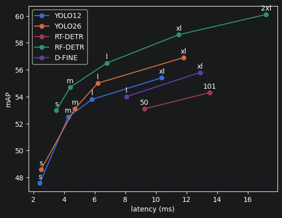
Benchmark comparison
To give a comparison between the models, here are the exact benchmark values. All scores on MS COCO val2017. Latency was measured on an NVIDIA T4 GPU.
| Model | mAP50 | mAP50:95 | Latency | Params | Edge-ready | License |
|---|---|---|---|---|---|---|
| RF-DETR-N | 67.6 | 48.4 | 2.3 ms | 30.5 M | Server GPU | Apache 2.0 |
| RF-DETR-M | 73.6 | 54.7 | 4.4 ms | 33.7 M | Server GPU | Apache 2.0 |
| RF-DETR-2XL | 78.5 | 60.1 | 17.2 ms | 126.9 M | Server GPU | PML 1.0 |
| YOLO12-N | 56.7 | 40.4 | 1.6 ms | 2.5 M | ARM / Mobile / Jetson | AGPL-3.0 |
| YOLO12-L | 70.7 | 53.8 | 5.83 ms | 26.5 M | Jetson / TensorRT | AGPL-3.0 |
| YOLO26-N | - | 40.1 | 1.7 ms | 2.4 M | ARM / Mobile / Jetson | AGPL-3.0 |
| YOLO26-X | - | 56.9 | 11.8 ms | 55.7 M | Jetson / TensorRT | AGPL-3.0 |
Here is a visualization of the above results alongside additional modern object detection models for a more holistic comparison:
Use-case guidance
Occluded objects: RF-DETR (M/L) is the clear choice. Its DINOv2 backbone models global context across the full image, making it significantly better than CNN-based models at finding partially hidden objects.
Small objects: RF-DETR uses multi-scale feature extraction. YOLO26 also includes STAL (small-target-aware label assignment), making it competitive for small objects on edge hardware.
Edge / mobile / Jetson: YOLO26-N or YOLO12-N. YOLO26 is the Ultralytics recommendation for Jetson Orin/Xavier, Snapdragon AI, and ARM CPUs. It has 43% faster CPU inference than YOLO11n at comparable accuracy.
Custom domain / fine-tuning: RF-DETR by a significant margin. DINOv2 pre-training means it adapts to new domains (medical, aerial, and industrial) faster and with less data than any other model here.
Licensing Summary
| Model | License | Commercial use |
|---|---|---|
| RF-DETR (base) | Apache 2.0 | Free for all uses, including commercial products |
| RF-DETR XL/2XL | PML 1.0 | Contact Roboflow for commercial licensing |
| YOLO12 | AGPL-3.0 | Free for open source / personal use; commercial applications require an Ultralytics Enterprise license |
| YOLO26 | AGPL-3.0 | Free for open source / personal use; commercial applications require an Ultralytics Enterprise license |
Quick-start code
RF-DETR
# Install
pip install rfdetr

# Inference
from rfdetr import RFDETRBase
model = RFDETRBase()
detections = model.predict("image.jpg")

# Fine-tune on your dataset
model.train(dataset_dir="./my_dataset", epochs=50, batch_size=4)
YOLO26 / YOLO12 (via Ultralytics)
# Install
pip install ultralytics

# Inference - YOLO26
from ultralytics import YOLO
model = YOLO("yolo26n.pt")          # or yolo26s/m/l/x
results = model.predict("image.jpg")

# Inference - YOLO12
model = YOLO("yolo12n.pt")
results = model.predict("image.jpg")

# Export for edge (TensorRT / CoreML / ONNX)
model.export(format="engine")       # TensorRT for Jetson
model.export(format="coreml")       # Apple Silicon / iOS
model.export(format="tflite")       # Android / ARM
YOLO12 (use original open-source repo - not the Ultralytics integration)
# Install from the original authors' repo
conda create -n yolov12 python=3.11
conda activate yolov12
git clone https://github.com/sunsmarterjie/yolov12 && cd yolov12
pip install -r requirements.txt
pip install -e .

# Inference
from ultralytics import YOLO
model = YOLO("yolov12n.pt")         # or s/m/l/x
results = model("path/to/image.jpg")
results[0].show()

# Export for edge
model.export(format="engine", half=True)   # TensorRT FP16
model.export(format="onnx")                # ONNX for broad compatibility
Transfer learning and fine-tuning
RF-DETR - recommended for domain shift. Thanks to a DINOv2 backbone that is pre-trained on internet-scale data, fine-tuning requires less labeled data and converges faster. Use the rfdetr package with a COCO pre-trained checkpoint. Roboflow also offers a hosted fine-tuning UI.
YOLO26 / YOLO12 - easiest pipeline. Ultralytics' training API is the most mature fine-tuning ecosystem. It supports YOLO-format and COCO-format datasets and has good documentation and an active community.
# Fine-tuning YOLO26 on a custom dataset (YOLO format)
from ultralytics import YOLO

model = YOLO("yolo26m.pt")          # start from pretrained weights
model.train(
    data="custom_dataset.yaml",     # path to your dataset config
    epochs=100,
    imgsz=640,
    batch=16,
    device=0,                       # GPU index; "cpu" for CPU
)
metrics = model.val()               # evaluate on validation set
Summary: Choosing the right model for your project
Selecting an object detection model requires matching your specific requirements against each model's strengths. The decision framework below maps common scenarios to optimal model choices.
| Your goal | Best choice | Runner-up |
|---|---|---|
| Highest accuracy, cloud deployment | RF-DETR M/XL | YOLO26-X |
| Edge / Jetson / mobile | YOLO26-N/S | YOLO12-N |
| Fine-tuning on a custom domain | RF-DETR | YOLO26 |
| Occluded / complex scenes | RF-DETR | YOLO26 |
| Research / benchmarking | YOLO12 | RF-DETR |
| Apache 2.0 + commercial use | RF-DETR (base) | YOLO26 |
| Multi-task (detect + segment + pose) | YOLO26 | RF-DETR (det+seg) |
Get started with PyCharm today
Selecting an object detection architecture in 2026 is a strategic decision dictated by the specific requirements of the application and the available computational budget. Whether prioritizing the record-breaking accuracy of RF-DETR for complex scenes or the unmatched efficiency of the YOLO family for edge deployment, the choice must balance mAP requirements against real-time latency constraints.
The landscape of computer vision is rapidly shifting toward zero-shot detection frameworks that recognize novel objects without task-specific supervision. As foundation models increasingly integrate sophisticated image embedders like CLIP or DINOv2 into detection pipelines, the boundaries of high-precision detection on resource-constrained hardware will continue to expand. While transformer-based architectures are developing quickly, the YOLO family's established ecosystem ensures it remains a cornerstone for real-time production environments.
To achieve the best results for your specific use case, we encourage you to experiment with the models and code samples provided in this guide. To that end, PyCharm provides the perfect ecosystem for experimentation with various open-source models via Code -> Insert HF Model interface. If you'd like to try this yourself, PyCharm Pro comes with a 30-day trial.
For a hands-on starting point, this tutorial shows how to build a live object detection app using TensorFlow and PyCharm Jupyter notebooks, then deploy it on a robot - covering everything from single-frame inference to a live web dashboard with annotated detections. Moreover, stay tuned for the next tutorial post, where we will discuss all three object detection models in action.
07 Jul 2026 5:51pm GMT
Ari Lamstein: This Thursday: Building Data Apps with Streamlit and Copilot
On July 9 (9am-1pm Pacific) - this Thursday - I'll be teaching a 4-hour live workshop for O'Reilly: Building Data Apps with Streamlit and Copilot.
This is the second time I've run this workshop, and I've made several improvements based on what I learned the first time.
If you work in Python and want to turn your analyses into interactive, shareable tools, this workshop is designed for you. We'll start from a Jupyter notebook and build a complete Streamlit app that lets users explore a dataset through interactive controls, charts, and maps. Along the way, you'll also learn to use Copilot as a companion while developing software - everything from learning the library faster to improving the quality of the code you write.
What we'll cover
- Structuring a Streamlit app
- Working with user input (select boxes, filters, etc.)
- Creating interactive graphics with Plotly
- Organizing the UI with columns and tabs
- Deploying your app to Streamlit Cloud
The workshop is hands-on: you'll build the app step-by-step, and by the end you'll have a working project you can adapt to your own data.
What You'll Build
Here's a screenshot from the app we'll build together:

The app lets users choose a state and demographic statistic, explore how it changes over time, and view the data as a chart, map, or table.
And while the example uses demographic data, the skills you'll learn - structuring an app, building interactive controls, and creating dynamic visualizations - apply to any Streamlit project you want to build.
Who is this for?
- Data scientists and analysts who want to make their work more interactive
- Python users who want to build dashboards without learning web development
- Anyone curious about Streamlit or Copilot
How to Register
The workshop is hosted on O'Reilly, which is a membership platform. If you're not already a member, O'Reilly offers a free 10-day trial - plenty of time to register and attend this week.
Also worth knowing: the workshop is recorded. So if July 9 doesn't work for you, it's still worth registering - you'll have access to the recording.
I'd love to see you there.
07 Jul 2026 4:00pm GMT
Django Weblog: Django security releases issued: 6.0.7 and 5.2.16
In accordance with our security release policy, the Django team is issuing releases for Django 6.0.7 and Django 5.2.16. These releases address the security issues detailed below. We encourage all users of Django to upgrade as soon as possible.
CVE-2026-48588: Potential exposure of private data via cached Set-Cookie response
django.middleware.cache.UpdateCacheMiddleware and django.views.decorators.cache.cache_page avoided caching responses that set a cookie while varying on Cookie only when the incoming request contained no cookies at all. When the request already carried an unrelated cookie (such as a language or theme preference cookie), the protection did not apply, allowing a response that sets a session or other sensitive cookie to be stored in Django's shared cache.
This issue has severity "low" according to the Django security policy.
Thanks to Chris Whyland for the report.
CVE-2026-53877: Heap buffer over-read in GDALRaster
When django.contrib.gis.gdal.GDALRaster was instantiated with a bytes object representing a raster file, the vsi_buffer property could over-read the allocated buffer by approximately 32 bytes. This could result in information disclosure of adjacent heap memory or, in rare cases, a segmentation fault. Only rasters stored in GDAL's virtual filesystem were affected.
This issue has severity "low" according to the Django security policy.
Thanks to Bence Nagy for the report.
CVE-2026-53878: Header injection possibility since DomainNameValidator accepted newlines in input
django.core.validators.DomainNameValidator accepted newlines in domain names. If such values were included in HTTP responses, header injection attacks were possible. Django itself wasn't vulnerable because HttpResponse prohibits newlines in HTTP headers.
The vulnerability only affected uses of DomainNameValidator outside Django form fields, as CharField strips newlines by default.
This issue has severity "low" according to the Django security policy.
Thanks to Bence Nagy for the report.
Affected supported versions
- Django main
- Django 6.1 (currently at beta status)
- Django 6.0
- Django 5.2
Resolution
Patches to resolve the issue have been applied to Django's main, 6.1 (currently at beta status), 6.0, and 5.2 branches. The patches may be obtained from the following changesets.
CVE-2026-48588: Potential exposure of private data via cached Set-Cookie response
- On the main branch
- On the 6.1 branch
- On the 6.0 branch
- On the 5.2 branch
CVE-2026-53877: Heap buffer over-read in GDALRaster
- On the main branch
- On the 6.1 branch
- On the 6.0 branch
- On the 5.2 branch
CVE-2026-53878: Header injection possibility since DomainNameValidator accepted newlines in input
- On the main branch
- On the 6.1 branch
- On the 6.0 branch
- On the 5.2 branch
The following releases have been issued
The PGP key ID used for this release is Jacob Walls: 131403F4D16D8DC7
General notes regarding security reporting
As always, we ask that potential security issues be reported via private email to security@djangoproject.com, and not via Django's Trac instance, nor via the Django Forum. Please see our security policies for further information.
07 Jul 2026 2:00pm GMT
PyCon: Welcome, Kattni!

Everyone has different reasons for attending PyCon US; the event has a wide range of things to offer. For me, it's about the people -- seeing old friends and making new ones is by far my favorite part of the conference. I want to focus on helping the PyCon US community grow, to further cultivate the myriad perspectives, and increase the opportunities for everyone involved to have their own amazing and memorable experiences. When it comes down to it, PyCon US happens at all because of those who participate. It wouldn't exist without, at a very minimum, those who: organise it, run it, volunteer both before and during, submit to the CFP, speak, teach tutorials, present posters, sponsor, and attend.
I hope you'll join us next year in Long Beach, as I begin my journey helping make PyCon US a wonderful event. I'm incredibly excited to be working alongside Jon, and the rest of the staff, organisers, and volunteers, through the next four years. I'm looking forward to seeing everyone next year!
We'll have more news to share about PyCon US 2027 in the coming months. Stay tuned to the blog and newsletter for updates. We look forward to welcoming you back to Long Beach next May 12 - 18.
07 Jul 2026 11:50am GMT
Python Bytes: #487 Minimum requirements
<strong>Topics covered in this episode:</strong><br> <ul> <li><strong><a href="https://github.com/bootandy/dust?featured_on=pythonbytes">dust</a> - a better du</strong></li> <li><strong><a href="https://hermes-agent.org/?featured_on=pythonbytes">Hermes Agent</a>: The AI agent that grows with you</strong></li> <li><strong><a href="https://github.com/simonw/llm-coding-agent/releases/tag/0.1a0?featured_on=pythonbytes">llm-coding-agent 0.1a0</a></strong></li> <li><strong>Extras</strong></li> <li><strong>Joke</strong></li> </ul><a href='https://www.youtube.com/watch?v=KubyT7Ttggg' style='font-weight: bold;'data-umami-event="Livestream-Past" data-umami-event-episode="487">Watch on YouTube</a><br> <p><strong>About the show</strong></p> <p>Sponsored by us! Support our work through:</p> <ul> <li>Our <a href="https://training.talkpython.fm/?featured_on=pythonbytes"><strong>courses at Talk Python</strong></a></li> <li>Consulting from <a href="https://sixfeetup.com/?featured_on=pythonbytes"><strong>Six Feet Up</strong></a></li> </ul> <p><strong>Connect with the hosts</strong></p> <ul> <li>Michael: <a href="https://fosstodon.org/@mkennedy">Mastodon</a> / <a href="https://bsky.app/profile/mkennedy.codes?featured_on=pythonbytes">BlueSky</a> / <a href="https://x.com/mkennedy?featured_on=pythonbytes">X</a> / <a href="https://www.linkedin.com/in/mkennedy/?featured_on=pythonbytes">LinkedIn</a></li> <li>Calvin: <a href="https://sixfeetup.social/@calvin?featured_on=pythonbytes">Mastodon</a> / <a href="https://bsky.app/profile/calvinhp.com?featured_on=pythonbytes">BlueSky</a> / <a href="https://x.com/calvinhp?featured_on=pythonbytes">X</a> / <a href="https://www.linkedin.com/in/calvinhp/?featured_on=pythonbytes">LinkedIn</a></li> <li>Show: <a href="https://fosstodon.org/@pythonbytes">Mastodon</a> / <a href="https://bsky.app/profile/pythonbytes.fm">BlueSky</a> / <a href="https://x.com/PythonBytes?featured_on=pythonbytes">X</a></li> </ul> <p>Join us on YouTube at <a href="https://pythonbytes.fm/stream/live"><strong>pythonbytes.fm/live</strong></a> to be part of the audience. Usually <strong>Tuesday at 7am PT</strong>. Older video versions available there too.</p> <p>Finally, if you want an artisanal, hand-crafted digest of every week of the show notes in email form? Add your name and email to <a href="https://pythonbytes.fm/friends-of-the-show">our friends of the show list</a>, we'll never share it.</p> <p><strong>Michael #1: <a href="https://github.com/bootandy/dust?featured_on=pythonbytes">dust</a> -</strong> a better du</p> <ul> <li><code>du</code> + Rust = <code>dust</code> - a fast, visual, intuitive disk-usage CLI</li> <li>Run <code>dust</code> and immediately see the biggest directories and files without piping through <code>sort</code>, <code>head</code>, or <code>awk</code></li> <li>Smart recursive output focuses on what matters instead of dumping every folder</li> <li>Colored bars show relative size and parent/child hierarchy, making "where did the space go?" obvious</li> <li>Perfect for Python projects bloated by <code>.venv</code>, caches, Docker volumes, downloaded datasets, and local AI models</li> <li>Install via <code>brew</code>, <code>cargo install du-dust</code>, <code>conda-forge</code>, Scoop, Snap, deb-get, or GitHub releases</li> </ul> <p><strong>Calvin #2</strong>: <a href="https://github.com/astral-sh/war/blob/main/SPEC.md?featured_on=pythonbytes">A Way better ARchive format for Python packaging</a></p> <ul> <li><strong>war</strong> - new archive format spec from Astral (same team as uv/ruff), v0.0.2, still no binary encoding defined yet</li> <li>Header-Index-Store layout: header IDs the file, index maps names to store offsets, store holds compressed data</li> <li>Index uses a finite-state transducer (FST) to dedupe common path prefixes across entry names</li> <li>Supports three entry types (file, directory, link) and three compression modes (store/DEFLATE/zstd), plus an "executable" metadata flag</li> <li>Unpacking is atomic - writes to a temp dir, then renames into place, so a failed extract never leaves a half-unpacked directory</li> <li>Strict name-segment rules (no NUL/control chars, no leading/trailing whitespace, blocks Windows-reserved names like CON/PRN) to avoid path traversal and cross-platform footguns</li> </ul> <p><strong>Michael #3:</strong> <a href="https://hermes-agent.org/?featured_on=pythonbytes">Hermes Agent</a>: The AI agent that grows with you</p> <ul> <li>Hermes Agent is an open-source, Python-built AI agent framework from Nous Research - think ChatGPT-style assistant, but connected to your tools, files, shell, browser, calendar, memory, and messaging apps</li> <li>I'm using it in Discord as a long-running agent conversation, not just a one-off chatbot session</li> <li>Hermes can connect through a gateway to platforms like Discord, Telegram, Slack, WhatsApp, email, webhooks, and more - so the same assistant can follow you across surfaces</li> <li>In my setup, I can send Hermes voice/text from Discord, keep project context across turns as threads, and ask it to actually do things: read GitHub repos, run commands, edit files, schedule calendar events, generate drafts, and verify results</li> <li>A fun workflow: I can trigger one-shot actions from an Apple Watch shortcut - dictate a request, send it to Hermes, and have the agent execute it asynchronously</li> <li>Hermes has persistent memory, so it can remember durable preferences and facts - for example, how I like my research formatted</li> <li>It also has "skills," which are reusable procedures the agent can load later, so Hermes can self-improve over time instead of rediscovering the same workflow repeatedly</li> <li>It supports scheduled jobs / cron-style automations, so it can proactively watch for releases, send summaries, run checks, or remind you about things</li> <li>It's provider-agnostic: OpenRouter, Anthropic, Google, xAI, local models, Nous Portal, and others</li> <li>The big idea: Hermes turns an LLM from "a chat box I visit" into "an agent I can reach from anywhere that knows my workflows and can take real actions and learns over time."</li> </ul> <p><strong>Calvin #4: <a href="https://github.com/simonw/llm-coding-agent/releases/tag/0.1a0?featured_on=pythonbytes">llm-coding-agent 0.1a0</a></strong></p> <ul> <li>Simon Willison built a Claude/Codex-style coding agent on top of his <code>llm</code> library, using an alpha of the <code>llm</code> package plus his python-lib-template-repo</li> <li>Built almost entirely via prompted TDD - asked an agent to write a <a href="http://spec.md?featured_on=pythonbytes">spec.md</a>, then commit + implement with red/green tests, occasionally hitting a real OpenAI key to sanity-check</li> <li>Shipped to PyPI as an alpha: <code>uvx --prerelease=allow --with llm-coding-agent llm code</code></li> <li>Tool set mirrors familiar coding-agent primitives: read_file, edit_file (exact string replace + diff), write_file, list_files, search_files, execute_command</li> <li>Also exposes a Python API - <code>CodingAgent(model="gpt-5.5", root=..., approve=True).run(...)</code> - which Simon didn't ask for but got anyway</li> <li>Demo: <code>llm code --yolo</code> told GPT-5.5 to build a SwiftUI CLI clock; model correctly noted SwiftUI isn't really CLI-friendly and still produced an ASCII-art time display</li> </ul> <p><strong>Extras</strong></p> <p>Calvin:</p> <ul> <li>Slides, but for developers <a href="https://sli.dev/?featured_on=pythonbytes">https://sli.dev/</a></li> <li>Wanna reduce your token usage…. only issue is that its lossy <a href="https://github.com/teamchong/pxpipe?featured_on=pythonbytes">https://github.com/teamchong/pxpipe</a></li> <li><strong>PEP 772 - Python Packaging Council inaugural election dates set, nominations open July 28, voting September 1-15</strong></li> </ul> <p>Michael:</p> <ul> <li><a href="https://mkennedy.codes/posts/what-the-pls/?featured_on=pythonbytes">What the pls?</a> revisited!</li> </ul> <p><strong>Joke:</strong> <a href="https://x.com/AlfinCodes/status/2057443209127903456?featured_on=pythonbytes">Min requirements for Linux</a></p>
07 Jul 2026 8:00am GMT